Sono un ricercatore di intelligenza artificiale, quindi una delle cose principali di cui mi occupo sono i dati. Un molto di esso.
Con oltre 2,5 exabyte di dati generati ogni giorno , non sorprende che questi dati debbano essere archiviati in un luogo dove possiamo accedervi quando ne abbiamo bisogno.
Questo articolo ti guiderà attraverso un cheatsheet hackerabile per metterti rapidamente in funzione con SQL.
Cos'è SQL?
SQL sta per Structured Query Language. È un linguaggio per i sistemi di gestione di database relazionali. SQL viene utilizzato oggi per archiviare, recuperare e manipolare i dati all'interno di database relazionali.
Ecco come appare un database relazionale di base:
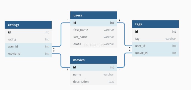
Utilizzando SQL, possiamo interagire con il database scrivendo query.
Ecco come appare una query di esempio:
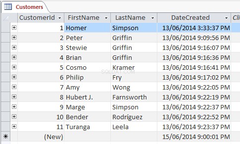
SELECT * FROM customers;
Usando questo SELECT istruzione, la query seleziona tutti i dati di tutte le colonne nella tabella del cliente e restituisce i dati in questo modo:
Il carattere jolly asterisco (*) si riferisce a "tutti ” e seleziona tutti le righe e le colonne. Possiamo invece sostituirlo con nomi di colonne specifici — qui solo quelle colonne verranno restituite dalla query
SELECT FirstName, LastName FROM customers;
Aggiunta di un WHERE La clausola consente di filtrare ciò che viene restituito:
SELECT * FROM customers WHERE age >= 30 ORDER BY age ASC;Questa query restituisce tutti i dati dalla tabella dei prodotti con un'età valore maggiore di 30.
L'uso di ORDER BY parola chiave significa semplicemente che i risultati verranno ordinati utilizzando la colonna dell'età dal valore più basso al più alto
Usando il INSERT INTO istruzione, possiamo aggiungere nuovi dati a una tabella. Ecco un esempio di base per aggiungere un nuovo utente alla tabella clienti:
INSERT INTO customers(FirstName, LastName, address, email)
VALUES ('Jason', 'Dsouza', 'McLaren Vale, South Australia', 'test@fakeGmail.com');
Naturalmente, questi esempi dimostrano solo una selezione molto piccola di ciò che può fare il linguaggio SQL. Ne sapremo di più in questa guida.
Perché imparare l'SQL?
Viviamo nell'era dei Big Data, in cui i dati vengono ampiamente utilizzati per trovare approfondimenti e informare su strategie, marketing, pubblicità e una miriade di altre operazioni.
Le grandi aziende come Google, Amazon, AirBnb utilizzano database relazionali di grandi dimensioni come base per migliorare l'esperienza del cliente. Comprendere SQL è una grande abilità non solo per i data scientist e gli analisti, ma per tutti.
Come pensi di aver improvvisamente ricevuto un annuncio su Youtube sulle scarpe quando solo pochi minuti fa stavi cercando su Google le tue scarpe preferite? Questo è SQL (o una forma di SQL) al lavoro!
SQL vs MySQL
Prima di andare avanti, voglio solo chiarire un argomento spesso confuso — la differenza tra SQL e MySQL. A quanto pare, non lo sono la stessa cosa!
SQL è un linguaggio, mentre MySQL è un sistema per implementare SQL.
SQL delinea la sintassi che consente di scrivere query che gestiscono database relazionali.
MySQL è un sistema di database che gira su un server. Ti consente di scrivere query utilizzando la sintassi SQL per gestire i database MySQL.
Oltre a MySQL, esistono altri sistemi che implementano SQL. Alcuni dei più popolari includono:
- SQLite
- Database Oracle
- PostgreSQL
- Microsoft SQL Server
Come installare MySQL
Nella maggior parte dei casi, MySQL è la scelta preferita per un sistema di gestione di database. Molti sistemi di gestione dei contenuti popolari (come Wordpress) utilizzano MySQL per impostazione predefinita, quindi utilizzare MySQL per gestire tali applicazioni può essere una buona idea.
Per utilizzare MySQL, devi installarlo sul tuo sistema:
Installa MySQL su Windows
Il modo consigliato per installare MySQL su Windows è utilizzare il programma di installazione MSI dal sito Web MySQL.
Questa risorsa ti guiderà nel processo di installazione.
Installa MySQL su macOS
Su macOS, l'installazione di MySQL implica anche il download di un programma di installazione.
Questa risorsa ti guiderà attraverso il processo di installazione.
Come utilizzare MySQL
Con MySQL ora installato sul tuo sistema, ti consiglio di utilizzare una sorta di applicazione di gestione SQL per semplificare notevolmente la gestione dei database.
Ci sono molte app tra cui scegliere che svolgono in gran parte lo stesso lavoro, quindi dipende dalle tue preferenze personali su quale utilizzare:
- MySQL Workbench sviluppato da Oracle
- phpMyAdmin (funziona nel browser web)
- HeidiSQL (consigliato per Windows)
- Sequel Pro (consigliato per macOS)
Quando sei pronto per iniziare a scrivere le tue query SQL, prendi in considerazione l'importazione di dati fittizi anziché creare il tuo database.
Ecco alcuni database fittizi che possono essere scaricati gratuitamente.
SQL Cheatsheet – La ciliegina sulla torta
Parole chiave SQL
Qui puoi trovare una raccolta di parole chiave utilizzate nelle istruzioni SQL, una descrizione e, se del caso, un esempio. Alcune delle parole chiave più avanzate hanno una propria sezione dedicata.
Laddove MySQL è menzionato accanto a un esempio, significa che questo esempio è applicabile solo ai database MySQL (al contrario di qualsiasi altro sistema di database).
ADD -- Adds a new column to an existing table

ADD CONSTRAINT -- Creates a new constraint on an existing table, which is used to specify rules for any data in the table.

ALTER TABLE -- Adds, deletes or edits columns in a table. It can also be used to add and delete constraints in a table, as per the above.

ALTER COLUMN -- Changes the data type of a table’s column.

ALL -- Returns true if all of the subquery values meet the passed condition.

AND -- Used to join separate conditions within a WHERE clause.

ANY -- Returns true if any of the subquery values meet the given condition.

AS -- Renames a table or column with an alias value which only exists for the duration of the query.

ASC -- Used with ORDER BY to return the data in ascending order.

BETWEEN -- Selects values within the given range.

CASE -- Changes query output depending on conditions.

CHECK -- Adds a constraint that limits the value which can be added to a column.

CREATE DATABASE -- Creates a new database.

CREATE TABLE -- Creates a new table.

DEFAULT -- Sets a default value for a column

DELETE -- Delete data from a table.

DESC -- Used with ORDER BY to return the data in descending order.

DROP COLUMN -- Deletes a column from a table.

DROP DATABASE -- Deletes the entire database.

DROP DEAFULT -- Removes a default value for a column.

DROP TABLE -- Deletes a table from a database.

EXISTS -- Checks for the existence of any record within the subquery, returning true if one or more records are returned.

FROM -- Specifies which table to select or delete data from.

IN --  Used alongside a WHERE clause as a shorthand for multiple OR conditions.

INSERT INTO -- Adds new rows to a table.

IS NULL -- Tests for empty (NULL) values.

IS NOT NULL -- The reverse of NULL. Tests for values that aren’t empty / NULL.

LIKE -- Returns true if the operand value matches a pattern.

NOT -- Returns true if a record DOESN’T meet the condition.

OR -- Used alongside WHERE to include data when either condition is true.

ORDER BY -- Used to sort the result data in ascending (default) or descending order through the use of ASC or DESC keywords.

ROWNUM -- Returns results where the row number meets the passed condition.

SELECT -- Used to select data from a database, which is then returned in a results set.

SELECT DISTINCT -- Sames as SELECT, except duplicate values are excluded.

SELECT INTO -- Copies data from one table and inserts it into another.

SELECT TOP -- Allows you to return a set number of records to return from a table.

SET -- Used alongside UPDATE to update existing data in a table.

SOME -- Identical to ANY.

TOP -- Used alongside SELECT to return a set number of records from a table.

TRUNCATE TABLE -- Similar to DROP, but instead of deleting the table and its data, this deletes only the data.

UNION -- Combines the results from 2 or more SELECT statements and returns only distinct values.

UNION ALL -- The same as UNION, but includes duplicate values.

UNIQUE -- This constraint ensures all values in a column are unique.

UPDATE -- Updates existing data in a table.

VALUES -- Used alongside the INSERT INTO keyword to add new values to a table.

WHERE -- Filters results to only include data which meets the given condition.
Commenti in SQL
I commenti ti consentono di spiegare sezioni delle tue istruzioni SQL, senza essere eseguiti direttamente.
In SQL, ci sono 2 tipi di commenti, riga singola e multilinea.
Commenti a riga singola in SQL
I commenti a riga singola iniziano con '- -'. Qualsiasi testo dopo questi 2 caratteri fino alla fine della riga verrà ignorato.
-- This part is ignored

SELECT * FROM customers;
Commenti su più righe in SQL
I commenti su più righe iniziano con /* e terminano con */. Si estendono su più righe finché non vengono trovati i caratteri di chiusura.
/*

This is a multiline comment.
It can span across multiple lines.

*/

SELECT * FROM customers;

/*

This is another comment.
You can even put code within a comment to prevent its execution

SELECT * FROM icecreams;

*/
Tipi di dati in MySQL
Quando crei una nuova tabella o ne modifichi una esistente, devi specificare il tipo di dati che ogni colonna accetta.
In questo esempio, i dati sono passati a id la colonna deve essere un int (intero), mentre il FirstName la colonna ha un VARCHAR tipo di dati con un massimo di 255 caratteri.
CREATE TABLE customers(
id int,
FirstName varchar(255)
);
1. Tipi di dati stringa
CHAR(size) -- Fixed length string which can contain letters, numbers and special characters. The size parameter sets the maximum string length, from 0 – 255 with a default of 1.

VARCHAR(size) -- Variable length string similar to CHAR(), but with a maximum string length range from 0 to 65535.

BINARY(size) -- Similar to CHAR() but stores binary byte strings.

VARBINARY(size) -- Similar to VARCHAR() but for binary byte strings.

TINYBLOB -- Holds Binary Large Objects (BLOBs) with a max length of 255 bytes.

TINYTEXT -- Holds a string with a maximum length of 255 characters. Use VARCHAR() instead, as it’s fetched much faster.

TEXT(size) -- Holds a string with a maximum length of 65535 bytes. Again, better to use VARCHAR().

BLOB(size) -- Holds Binary Large Objects (BLOBs) with a max length of 65535 bytes.

MEDIUMTEXT -- Holds a string with a maximum length of 16,777,215 characters.

MEDIUMBLOB -- Holds Binary Large Objects (BLOBs) with a max length of 16,777,215 bytes.

LONGTEXT -- Holds a string with a maximum length of 4,294,967,295 characters.

LONGBLOB -- Holds Binary Large Objects (BLOBs) with a max length of 4,294,967,295 bytes.

ENUM(a, b, c, etc…) -- A string object that only has one value, which is chosen from a list of values which you define, up to a maximum of 65535 values. If a value is added which isn’t on this list, it’s replaced with a blank value instead.

SET(a, b, c, etc…) -- A string object that can have 0 or more values, which is chosen from a list of values which you define, up to a maximum of 64 values.
2. Tipi di dati numerici
BIT(size) -- A bit-value type with a default of 1. The allowed number of bits in a value is set via the size parameter, which can hold values from 1 to 64.

TINYINT(size) -- A very small integer with a signed range of -128 to 127, and an unsigned range of 0 to 255. Here, the size parameter specifies the maximum allowed display width, which is 255.

BOOL -- Essentially a quick way of setting the column to TINYINT with a size of 1. 0 is considered false, whilst 1 is considered true.

BOOLEAN	-- Same as BOOL.

SMALLINT(size) -- A small integer with a signed range of -32768 to 32767, and an unsigned range from 0 to 65535. Here, the size parameter specifies the maximum allowed display width, which is 255.

MEDIUMINT(size) -- A medium integer with a signed range of -8388608 to 8388607, and an unsigned range from 0 to 16777215. Here, the size parameter specifies the maximum allowed display width, which is 255.

INT(size) -- A medium integer with a signed range of -2147483648 to 2147483647, and an unsigned range from 0 to 4294967295. Here, the size parameter specifies the maximum allowed display width, which is 255.

INTEGER(size) -- Same as INT.

BIGINT(size) -- A medium integer with a signed range of -9223372036854775808 to 9223372036854775807, and an unsigned range from 0 to 18446744073709551615. Here, the size parameter specifies the maximum allowed display width, which is 255.

FLOAT(p) -- A floating point number value. If the precision (p) parameter is between 0 to 24, then the data type is set to FLOAT(), whilst if it's from 25 to 53, the data type is set to DOUBLE(). This behaviour is to make the storage of values more efficient.

DOUBLE(size, d) -- A floating point number value where the total digits are set by the size parameter, and the number of digits after the decimal point is set by the d parameter.

DECIMAL(size, d) -- An exact fixed point number where the total number of digits is set by the size parameters, and the total number of digits after the decimal point is set by the d parameter.

DEC(size, d) -- Same as DECIMAL.
3. Tipi di dati data/ora
DATE -- A simple date in YYYY-MM–DD format, with a supported range from ‘1000-01-01’ to ‘9999-12-31’.

DATETIME(fsp) -- A date time in YYYY-MM-DD hh:mm:ss format, with a supported range from ‘1000-01-01 00:00:00’ to ‘9999-12-31 23:59:59’. By adding DEFAULT and ON UPDATE to the column definition, it automatically sets to the current date/time.

TIMESTAMP(fsp) -- A Unix Timestamp, which is a value relative to the number of seconds since the Unix epoch (‘1970-01-01 00:00:00’ UTC). This has a supported range from ‘1970-01-01 00:00:01’ UTC to ‘2038-01-09 03:14:07’ UTC.
By adding DEFAULT CURRENT_TIMESTAMP and ON UPDATE CURRENT TIMESTAMP to the column definition, it automatically sets to current date/time.

TIME(fsp) -- A time in hh:mm:ss format, with a supported range from ‘-838:59:59’ to ‘838:59:59’.

YEAR -- A year, with a supported range of ‘1901’ to ‘2155’.
Operatori SQL
1. Operatori aritmetici in SQL
+ -- Add
– -- Subtract
* -- Multiply
/ -- Divide
% -- Modulus
2. Operatori bit per bit in SQL
& -- Bitwise AND
| -- Bitwise OR
^-- Bitwise XOR
3. Operatori di confronto in SQL
= -- Equal to
> -- Greater than
< -- Less than
>= -- Greater than or equal to
<= -- Less than or equal to
<> -- Not equal to
4. Operatori composti in SQL
+= -- Add equals
-= -- Subtract equals
*= -- Multiply equals
/= -- Divide equals
%= -- Modulo equals
&= -- Bitwise AND equals
^-= -- Bitwise exclusive equals
|*= -- Bitwise OR equals
Funzioni SQL
1. Funzioni di stringa in SQL
ASCII -- Returns the equivalent ASCII value for a specific character.

CHAR_LENGTH -- Returns the character length of a string.

CHARACTER_LENGTH -- Same as CHAR_LENGTH.

CONCAT -- Adds expressions together, with a minimum of 2.

CONCAT_WS -- Adds expressions together, but with a separator between each value.

FIELD -- Returns an index value relative to the position of a value within a list of values.

FIND IN SET -- Returns the position of a string in a list of strings.

FORMAT -- When passed a number, returns that number formatted to include commas (eg 3,400,000).

INSERT -- Allows you to insert one string into another at a certain point, for a certain number of characters.

INSTR -- Returns the position of the first time one string appears within another.

LCASE -- Converts a string to lowercase.

LEFT -- Starting from the left, extracts the given number of characters from a string and returns them as another.

LENGTH -- Returns the length of a string, but in bytes.

LOCATE -- Returns the first occurrence of one string within another,

LOWER -- Same as LCASE.

LPAD -- Left pads one string with another, to a specific length.

LTRIM -- Removes any leading spaces from the given string.

MID -- Extracts one string from another, starting from any position.

POSITION -- Returns the position of the first time one substring appears within another.

REPEAT -- Allows you to repeat a string

REPLACE -- Allows you to replace any instances of a substring within a string, with a new substring.

REVERSE	-- Reverses the string.

RIGHT -- Starting from the right, extracts the given number of characters from a string and returns them as another.

RPAD -- Right pads one string with another, to a specific length.

RTRIM -- Removes any trailing spaces from the given string.

SPACE -- Returns a string full of spaces equal to the amount you pass it.

STRCMP -- Compares 2 strings for differences

SUBSTR -- Extracts one substring from another, starting from any position.

SUBSTRING -- Same as SUBSTR

SUBSTRING_INDEX	-- Returns a substring from a string before the passed substring is found the number of times equals to the passed number.

TRIM --	Removes trailing and leading spaces from the given string. Same as if you were to run LTRIM and RTRIM together.

UCASE -- Converts a string to uppercase.

UPPER -- Same as UCASE.
2. Funzioni numeriche in SQL
ABS -- Returns the absolute value of the given number.

ACOS -- Returns the arc cosine of the given number.

ASIN -- Returns the arc sine of the given number.

ATAN -- Returns the arc tangent of one or 2 given numbers.

ATAN2 -- Returns the arc tangent of 2 given numbers.

AVG -- Returns the average value of the given expression.

CEIL -- Returns the closest whole number (integer) upwards from a given decimal point number.

CEILING -- Same as CEIL.

COS -- Returns the cosine of a given number.

COT -- Returns the cotangent of a given number.

COUNT -- Returns the amount of records that are returned by a SELECT query.

DEGREES -- Converts a radians value to degrees.

DIV -- Allows you to divide integers.

EXP -- Returns e to the power of the given number.

FLOOR -- Returns the closest whole number (integer) downwards from a given decimal point number.

GREATEST -- Returns the highest value in a list of arguments.

LEAST -- Returns the smallest value in a list of arguments.

LN -- Returns the natural logarithm of the given number.

LOG -- Returns the natural logarithm of the given number, or the logarithm of the given number to the given base.

LOG10 -- Does the same as LOG, but to base 10.

LOG2 -- Does the same as LOG, but to base 2.

MAX -- Returns the highest value from a set of values.

MIN -- Returns the lowest value from a set of values.

MOD -- Returns the remainder of the given number divided by the other given number.

PI -- Returns PI.

POW -- Returns the value of the given number raised to the power of the other given number.

POWER -- Same as POW.

RADIANS -- Converts a degrees value to radians.

RAND -- Returns a random number.

ROUND -- Rounds the given number to the given amount of decimal places.

SIGN -- Returns the sign of the given number.

SIN -- Returns the sine of the given number.

SQRT -- Returns the square root of the given number.

SUM -- Returns the value of the given set of values combined.

TAN -- Returns the tangent of the given number.

TRUNCATE -- Returns a number truncated to the given number of decimal places.
3. Funzioni di data in SQL
ADDDATE -- Adds a date interval (eg: 10 DAY) to a date (eg: 20/01/20) and returns the result (eg: 20/01/30).

ADDTIME -- Adds a time interval (eg: 02:00) to a time or datetime (05:00) and returns the result (07:00).

CURDATE -- Gets the current date.

CURRENT_DATE -- Same as CURDATE.

CURRENT_TIME -- Gest the current time.

CURRENT_TIMESTAMP -- Gets the current date and time.

CURTIME -- Same as CURRENT_TIME.

DATE -- Extracts the date from a datetime expression.

DATEDIFF -- Returns the number of days between the 2 given dates.

DATE_ADD -- Same as ADDDATE.

DATE_FORMAT -- Formats the date to the given pattern.

DATE_SUB -- Subtracts a date interval (eg: 10 DAY) to a date (eg: 20/01/20) and returns the result (eg: 20/01/10).

DAY -- Returns the day for the given date.

DAYNAME -- Returns the weekday name for the given date.

DAYOFWEEK -- Returns the index for the weekday for the given date.

DAYOFYEAR -- Returns the day of the year for the given date.

EXTRACT -- Extracts from the date the given part (eg MONTH for 20/01/20 = 01).

FROM DAYS -- Returns the date from the given numeric date value.

HOUR -- Returns the hour from the given date.

LAST DAY -- Gets the last day of the month for the given date.

LOCALTIME -- Gets the current local date and time.

LOCALTIMESTAMP -- Same as LOCALTIME.

MAKEDATE -- Creates a date and returns it, based on the given year and number of days values.

MAKETIME -- Creates a time and returns it, based on the given hour, minute and second values.

MICROSECOND -- Returns the microsecond of a given time or datetime.

MINUTE -- Returns the minute of the given time or datetime.

MONTH -- Returns the month of the given date.

MONTHNAME -- Returns the name of the month of the given date.

NOW -- Same as LOCALTIME.

PERIOD_ADD -- Adds the given number of months to the given period.

PERIOD_DIFF -- Returns the difference between 2 given periods.

QUARTER -- Returns the year quarter for the given date.

SECOND -- Returns the second of a given time or datetime.

SEC_TO_TIME -- Returns a time based on the given seconds.

STR_TO_DATE -- Creates a date and returns it based on the given string and format.

SUBDATE -- Same as DATE_SUB.

SUBTIME -- Subtracts a time interval (eg: 02:00) to a time or datetime (05:00) and returns the result (03:00).

SYSDATE -- Same as LOCALTIME.

TIME -- Returns the time from a given time or datetime.

TIME_FORMAT -- Returns the given time in the given format.

TIME_TO_SEC -- Converts and returns a time into seconds.

TIMEDIFF -- Returns the difference between 2 given time/datetime expressions.

TIMESTAMP -- Returns the datetime value of the given date or datetime.

TO_DAYS -- Returns the total number of days that have passed from ‘00-00-0000’ to the given date.

WEEK -- Returns the week number for the given date.

WEEKDAY -- Returns the weekday number for the given date.

WEEKOFYEAR -- Returns the week number for the given date.

YEAR -- Returns the year from the given date.

YEARWEEK -- Returns the year and week number for the given date.
4. Funzioni varie in SQL
BIN -- Returns the given number in binary.

BINARY -- Returns the given value as a binary string.

CAST -- Converst one type into another.

COALESCE -- From a list of values, returns the first non-null value.

CONNECTION_ID -- For the current connection, returns the unique connection ID.

CONV -- Converts the given number from one numeric base system into another.

CONVERT -- Converts the given value into the given datatype or character set.

CURRENT_USER -- Returns the user and hostname which was used to authenticate with the server.

DATABASE -- Gets the name of the current database.

GROUP BY -- Used alongside aggregate functions (COUNT, MAX, MIN, SUM, AVG) to group the results.

HAVING -- Used in the place of WHERE with aggregate functions.

IF -- If the condition is true it returns a value, otherwise it returns another value.

IFNULL -- If the given expression equates to null, it returns the given value.

ISNULL -- If the expression is null, it returns 1, otherwise returns 0.

LAST_INSERT_ID -- For the last row which was added or updated in a table, returns the auto increment ID.

NULLIF -- Compares the 2 given expressions. If they are equal, NULL is returned, otherwise the first expression is returned.

SESSION_USER -- Returns the current user and hostnames.

SYSTEM_USER -- Same as SESSION_USER.

USER -- Same as SESSION_USER.

VERSION -- Returns the current version of the MySQL powering the database.
Caratteri jolly in SQL
In SQL, i caratteri jolly sono caratteri speciali utilizzati con LIKE e NOT LIKE parole chiave. Questo ci consente di cercare dati con schemi sofisticati in modo piuttosto efficiente.
% -- Equates to zero or more characters.
-- Example: Find all customers with surnames ending in ‘ory’.
SELECT * FROM customers
WHERE surname LIKE '%ory';

_ -- Equates to any single character.
-- Example: Find all customers living in cities beginning with any 3 characters, followed by ‘vale’.
SELECT * FROM customers
WHERE city LIKE '_ _ _vale';

[charlist] -- Equates to any single character in the list.
-- Example: Find all customers with first names beginning with J, K or T.
SELECT * FROM customers
WHERE first_name LIKE '[jkt]%';
Chiavi SQL
Nei database relazionali esiste un concetto di primario e stranieri chiavi. Nelle tabelle SQL, questi sono inclusi come vincoli, in cui una tabella può avere una chiave primaria, una chiave esterna o entrambe.
1. Chiavi primarie in SQL
Un elemento primario consente di identificare in modo univoco ogni record in una tabella. Puoi avere solo una chiave primaria per tabella e puoi assegnare questo vincolo a qualsiasi singola o combinazione di colonne. Tuttavia, ciò significa che ogni valore all'interno di queste colonne deve essere univoco.
Tipicamente in una tabella, la colonna ID è una chiave primaria e di solito è accoppiata con AUTO_INCREMENT parola chiave. Ciò significa che il valore aumenta automaticamente man mano che vengono creati nuovi record.
Esempio (MySQL)
Crea una nuova tabella e imposta la chiave primaria sulla colonna ID.
CREATE TABLE customers (
id int NOT NULL AUTO_INCREMENT,
FirstName varchar(255),
Last Name varchar(255) NOT NULL,
address varchar(255),
email varchar(255),
PRIMARY KEY (id)
);
2. Chiavi esterne in SQL
Puoi applicare una chiave esterna a una o più colonne. Lo usi per collegare 2 tabelle insieme in un database relazionale.
La tabella contenente la chiave esterna è chiamata figlio chiave,
La tabella contenente la chiave di riferimento (o candidata) è chiamata parent tabella.
Ciò significa essenzialmente che i dati della colonna sono condivisi tra 2 tabelle, perché una chiave esterna impedisce anche l'inserimento di dati non validi che non sono presenti anche nella tabella padre.
Esempio (MySQL)
Crea una nuova tabella e trasforma qualsiasi colonna che fa riferimento a ID in altre tabelle in chiavi esterne.
CREATE TABLE orders (
id int NOT NULL,
user_id int,
product_id int,
PRIMARY KEY (id),
FOREIGN KEY (user_id) REFERENCES users(id),
FOREIGN KEY (product_id) REFERENCES products(id)
);
Indici in SQL
Gli indici sono attributi che possono essere assegnati a colonne che vengono spesso ricercate per rendere il recupero dei dati un processo più rapido ed efficiente.
CREATE INDEX -- Creates an index named ‘idx_test’ on the first_name and surname columns of the users table. In this instance, duplicate values are allowed.
CREATE INDEX idx_test
ON users (first_name, surname);
CREATE UNIQUE INDEX -- The same as the above, but no duplicate values.
CREATE UNIQUE INDEX idx_test
ON users (first_name, surname);
DROP INDEX -- Removes an index.
ALTER TABLE users
DROP INDEX idx_test;
Join SQL
In SQL, un JOIN La clausola viene utilizzata per restituire un risultato che combina i dati di più tabelle, sulla base di una colonna comune presente in entrambe.
Sono disponibili diversi join da utilizzare:
- Partecipazione interna (impostazione predefinita): Restituisce tutti i record che hanno valori corrispondenti in entrambe le tabelle.
- Partecipa a sinistra: Restituisce tutti i record della prima tabella, insieme a tutti i record corrispondenti della seconda tabella.
- Partecipa a destra: Restituisce tutti i record della seconda tabella, insieme a tutti i record corrispondenti della prima.
- Partecipazione completa: Restituisce tutti i record di entrambe le tabelle quando c'è una corrispondenza.
Un modo comune per visualizzare come funzionano i join è questo:

SELECT orders.id, users.FirstName, users.Surname, products.name as ‘product name’
FROM orders
INNER JOIN users on orders.user_id = users.id
INNER JOIN products on orders.product_id = products.id;
Viste in SQL
Una vista è essenzialmente un set di risultati SQL che viene archiviato nel database sotto un'etichetta, in modo da potervi tornare in un secondo momento senza dover eseguire nuovamente la query.
Questi sono particolarmente utili quando si dispone di una query SQL costosa che potrebbe essere necessaria un certo numero di volte. Quindi, invece di eseguirlo più e più volte per generare lo stesso set di risultati, puoi farlo solo una volta e salvarlo come vista.
Come creare viste in SQL
Per creare una vista, puoi farlo in questo modo:
CREATE VIEW priority_users AS
SELECT * FROM users
WHERE country = ‘United Kingdom’;
Quindi in futuro, se hai bisogno di accedere al set di risultati memorizzato, puoi farlo in questo modo:
SELECT * FROM [priority_users];Come sostituire le viste in SQL
Con il CREATE OR REPLACE comando, puoi aggiornare una vista come questa:
CREATE OR REPLACE VIEW [priority_users] AS
SELECT * FROM users
WHERE country = ‘United Kingdom’ OR country=’USA’;
Come eliminare le viste in SQL
Per eliminare una vista, usa semplicemente il DROP VIEW comando.
DROP VIEW priority_users;Conclusione
La maggior parte dei siti Web e delle applicazioni utilizza i database relazionali in un modo o nell'altro. Ciò rende SQL estremamente prezioso da conoscere in quanto consente di creare sistemi più complessi e funzionali.
Assicurati di seguirmi su Twitter per aggiornamenti su articoli futuri. Buon apprendimento!